Bioinformatics and AI: CNNs for bioinformatics
Published:
The corresponding notebook about the following article can directly be launched through google collab ![]()

DNA x AI | Pixabay
Bioinformatics and A.I: Let’s explore CNNs
Let’s dive into DNA sequences today! We’ll be using a dataset you can download from Kaggle: DNA Sequence Dataset. All the necessary files for this article are also available here.
In this dataset, you’ll find DNA sequences from three species: human, dog, and chimpanzee. Each sequence belongs to one of seven distinct gene families:
- 0: G protein-coupled receptors
- 1: Tyrosine kinase transmembrane receptors
- 2: Tyrosine phosphatase
- 3: Asparagine synthetase
- 4: Mitochondrial DNA
- 5: Vanilloid receptor
- 6: Homeodomain TF1
Our goal here is to tackle a multi-class classification problem, which differs from the binary classification we explored previously in this article: Bioinformatics and AI: A First Step.
We’ll need to encode these sequences so our neural network can analyze them. Today, I propose we use chaos theory (or chaos games), which we’ll delve into a bit later in this article. For now, let’s examine our data.
Exploratory Data Analysis (EDA)
We’ll focus on the human sequences, of which there are 4020. We’ll process these using a 5-mer representation (k=5), resulting in 32x32 pixel matrices.
\[representation = \sqrt{4^{k}}\]As with any machine learning approach, we’ll divide our dataset into three sets: training, test, and validation, following an 80%, 10%, and 10% split respectively. (For more information on data splitting, see here: Training, validation, and test sets). After resizing, we’ll obtain tensors of size 3216x32x32x1 for the training set and 402x32x32x1 for both the test and validation sets. This split will be stratified to maintain the proportions of the different classes.
Looking at the class distribution within the overall dataset, we observe an overrepresentation of sequences from class 0 and an underrepresentation of classes 3 and 6.
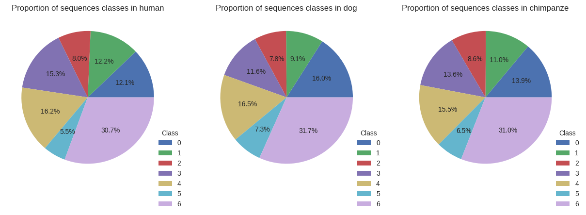
Repartition of every classes among datasets
Here’s the code for loading and preliminary exploring the data:
from collections import defaultdict
import numpy as np
import matplotlib.pyplot as plt
from matplotlib.gridspec import GridSpec
import pandas as pd

from sklearn.model_selection import train_test_split

import tensorflow as tf
import keras
from keras.datasets import mnist
from keras.layers import ZeroPadding2D, MaxPooling2D, Flatten
from tensorflow.keras.layers import Conv2D, Dense, Dropout, BatchNormalization, MaxPool2D
from tensorflow.keras.models import load_model
from keras.utils import to_categorical

# SVM part

from sklearn.datasets import make_classification
from sklearn.svm import SVC
from sklearn.metrics import accuracy_score

from sklearn.metrics import ConfusionMatrixDisplay

# Set plot styles
plt.style.use('seaborn-v0_8')

colors = plt.rcParams['axes.prop_cycle'].by_key()['color']
colors.append('#C8ADDF')


# Set tf seed
tf.random.set_seed(42)


"""# Mount drive"""

from google.colab import drive
drive.mount('/content/drive')

"""# Load data"""

working_folder = "/content/drive/MyDrive/Sequences/"

human_sequences = "/content/drive/MyDrive/Sequences/human.txt"
dog_sequences = "/content/drive/MyDrive/Sequences/dog.txt"
chimpanze_sequences = "/content/drive/MyDrive/Sequences/chimpanzee.txt"

df_human = pd.read_csv(human_sequences, sep = "\t")
df_dog = pd.read_csv(dog_sequences, sep = "\t")
df_chimpanze = pd.read_csv(chimpanze_sequences, sep = "\t")


# Exploratory Data Analysis

labels = [0 ,1, 2, 3, 4, 5, 6]
plt.figure(figsize = (15, 10))
plt.subplot(131)
plt.pie(df_human["class"].value_counts(sort = False).sort_index() , autopct='%1.1f%%', colors=colors)
plt.title("Proportion of sequences classes in human")
plt.legend(title="Class",
           labels=labels,
          loc="lower right", bbox_to_anchor=(1.1, -0.2))

plt.subplot(132)
labels_dog = df_dog["class"].unique()
plt.pie(df_dog["class"].value_counts(sort = False).sort_index() , autopct='%1.1f%%', colors=colors)
plt.title("Proportion of sequences classes in dog")
plt.legend(title="Class",
           labels=labels,
          loc="lower right", bbox_to_anchor=(1.1, -0.2))

plt.subplot(133)
labels_chimpanze = df_chimpanze["class"].unique()
plt.pie(df_chimpanze["class"].value_counts(sort = False).sort_index() , autopct='%1.1f%%', colors=colors)
plt.title("Proportion of sequences classes in chimpanze")
plt.legend(title="Class",
           labels=labels,
          loc="lower right", bbox_to_anchor=(1.1, -0.2))

plt.savefig(working_folder + "EDA.png", bbox_inches=‘tight’)
plt.show()
The Chaos Theory
Chaos theory, a field extensively studied in physics for many years, is closely linked to the creation of fractals (Wikipedia: Fractal).
In our case, we’ll create square matrix representations (graphics) of the sequences. These fractal-like representations are also intimately connected to the k-mer composition of our sequences. Let’s explore this in more detail.
To do this, we’ll define a square where each corner corresponds to one of the four fantastic nucleotides that enrich our field: A, T, C, and G. The center of the square will be our origin, (0, 0). Thus, we’ll place the four aforementioned nucleotides at the coordinates: A (-1, 1), G (1, 1), T (1, -1), and finally C (-1, -1).
The idea is to move within this square as we traverse the sequence. But how? It’s quite simple. Starting from the center of the square, we’ll move to the midpoint of the segment connecting our origin O(0, 0) to the first nucleotide of the sequence. Let’s take an example where T is the first nucleotide. We would then move to the midpoint between (0, 0) and (1, -1), which is (0.5, -0.5). Let’s call this point Q. Next, we head in the direction of the following nucleotide. If it’s a G, we’ll follow the segment connecting Q (0.5, -0.5) to G (1, 1) to reach the midpoint of that segment, which is point R (0.75, 0.25). The next nucleotide is an A. We then traverse the segment RA towards A (-1, 1) to the midpoint S (-0.125, 0.625), and so on…
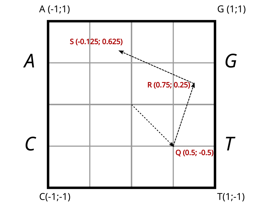
Chaos theory traveling path
This process places a set of points (one for each nucleotide in the sequence) within the initial square. The resulting representation will then reflect the abundance of all k-mers (for a predefined k).
Since numerical representations of spaces are discrete rather than continuous, we need to define our numerical space—in other words, the size of the output matrix. To do this, we must define the size k of the oligomers we’ll consider. The output matrix (or space) will then have a cardinality (or area) of \(4^k\) elements, forming a square with a side length of \(\sqrt{4^k}\).
The traversal method we just discussed allows us to locate k-mers within this matrix. Indeed, if we retrace the path, we first move towards the bottom-right quadrant of the square for ‘T’, then into the top-right quadrant of that previous quadrant for ‘G’, then into the top-left quadrant of that quadrant, and so on. With each nucleotide traversed, the current quadrant is re-divided into four, while preserving the orientations relative to the nucleotide vertices.
We’ll observe that all sequences, and by extension, all k-mers starting with ‘TG’, will be located in the top-right quadrant of the bottom-right quadrant. Following this successive division into four quadrants, it becomes possible to place all k-mers within the predefined space (or matrix elements, i.e., pixels of the image).
For a space representative of 2-mers and 3-mers, we would have the following divisions:
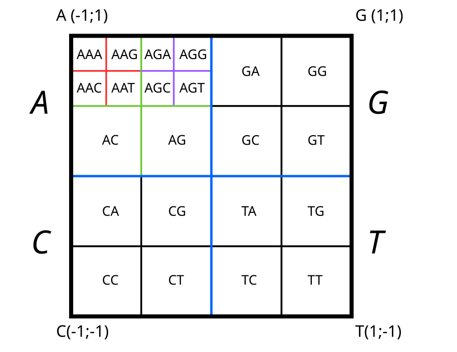
k-mers splitting inside CGR matrix
Alright, but what values should we assign to these quadrants or matrix elements? Well, now that the spaces dedicated to the k-mers are defined, we will assign to the corresponding elements in the matrix the probability of these k-mers appearing within the sequence. For more information on k-mers and calculating occurrence probabilities, you can refer to this link: Wikipedia: K-mer.
Thus, for a 3-mer representation, we would obtain an 8x8 dimension matrix whose elements would have a value between 0 and 1. For our tutorial, we’ll use 5-mers with a 32x32 representation.
To learn more about chaos theory representations, you can find information here.
The code required to produce such representations is as follows:
## Sanitize data
### Human
## Delete sequences that contains N
nb_sequences_to_drop = 0
rows_indexes_to_drop = list()
for idx, seq in enumerate(df_human['sequence']):
    if 'N' in seq :
      nb_sequences_to_drop +=1
      # display(df.loc[df['sequence'] == seq])
      rows_indexes_to_drop.append(idx)
print(f"Number of sequence to be dropped : {nb_sequences_to_drop}")
print(f"Rows to be dropped : {rows_indexes_to_drop}")
print(f"Shape of the data before dropping sequences containing Ns : {df_human.shape}")
df_human.drop(rows_indexes_to_drop, inplace = True)
print(f"Shape of the data after dropping sequences containing Ns : {df_human.shape}")

### Dog

nb_sequences_to_drop = 0
rows_indexes_to_drop = list()
for idx, seq in enumerate(df_dog['sequence']):
    if 'N' in seq :
      nb_sequences_to_drop +=1
      rows_indexes_to_drop.append(idx)
print(f"Number of sequence to be dropped : {nb_sequences_to_drop}")
print(f"Rows to be dropped : {rows_indexes_to_drop}")
print(f"Shape of the data before dropping sequences containing Ns : {df_dog.shape}")
df_dog = df_dog.drop(rows_indexes_to_drop, inplace = True)

### Chimpanze

nb_sequences_to_drop = 0
rows_indexes_to_drop = list()
for idx, seq in enumerate(df_chimpanze['sequence']):
    if 'N' in seq :
      nb_sequences_to_drop +=1
      rows_indexes_to_drop.append(idx)
print(f"Number of sequence to be dropped : {nb_sequences_to_drop}")
print(f"Rows to be dropped : {rows_indexes_to_drop}")
print(f"Shape of the data before dropping sequences containing Ns : {df_human.shape}")
df_chimpanze.drop(rows_indexes_to_drop, inplace = True)

## CGR transformation

def cgr_encoding(sequence: str, k: int) -> tf.Tensor:
  """
  sequence : Sequence to encode as CGR
  k = k-mers size
  """

  kmer_count = defaultdict(int)
  for i in range(len(sequence)-(k-1)):
      kmer_count[str(sequence[i :i+k])] +=1
  for key in kmer_count.keys():
      if "N" in key :
          del kmer_count[key]
  probabilities = defaultdict(float)
  N = len(sequence)
  for key, value in kmer_count.items():
      probabilities[key] = float(value) / (N - k + 1)
  array_size = int(np.sqrt(4**k))
  chaos = []
  for i in range(array_size):
      chaos.append([0]*array_size)
  maxx = array_size
  maxy = array_size
  posx = 1
  posy = 1
  for key, value in probabilities.items():
      for char in key :
          if char == "T":
              posx += maxx / 2
          elif char == "C":
              posy += maxy / 2
          elif char == "G":
              posx += maxx / 2
              posy += maxy / 2
          maxx = maxx / 2
          maxy /= 2
      chaos[int(posy)-1][int(posx)-1] = value
      maxx = array_size
      maxy = array_size
      posx = 1
      posy = 1
  return tf.constant(chaos)
>>> Number of sequence to be dropped : 360
>>> Shape of the data before dropping sequences containing Ns : (4380, 2)
>>> Shape of the data after dropping sequences containing Ns : (4020, 2)
>>> Number of sequence to be dropped : 17
>>> Rows to be dropped : [39, 49, 84, 95, 117, 165, 194, 198, 268, 299, 338, 342, 402, 628, 662, 757, 818]
>>> Shape of the data before dropping sequences containing Ns : (820, 2)
>>> Number of sequence to be dropped : 2
>>> Rows to be dropped : [134, 788]
>>> Shape of the data before dropping sequences containing Ns : (4020, 2)
Here’s what our sequences look like (no, no, it’s not a TV with bad reception).
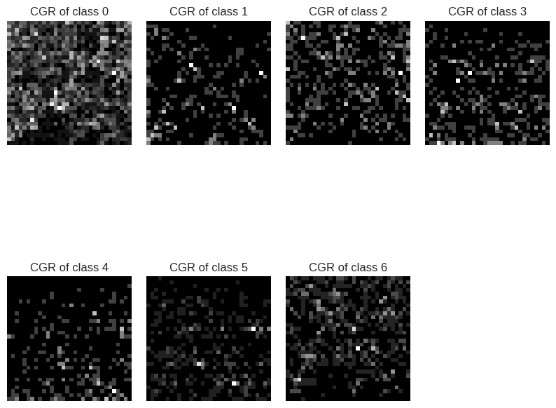
CGR representation for all the 6 classes
Here’s the code needed to produce these images:
## Plot data
# Randomly selected one example per class
random_idx_class_0 = np.random.choice(df_human[df_human["class"] == 0].index)
random_idx_class_1 = np.random.choice(df_human[df_human["class"] == 1].index)
random_idx_class_2 = np.random.choice(df_human[df_human["class"] == 2].index)
random_idx_class_3 = np.random.choice(df_human[df_human["class"] == 3].index)
random_idx_class_4 = np.random.choice(df_human[df_human["class"] == 4].index)
random_idx_class_5 = np.random.choice(df_human[df_human["class"] == 5].index)
random_idx_class_6 = np.random.choice(df_human[df_human["class"] == 6].index)

# Plot some data
fig= plt.figure(figsize=(10, 10))

gs = GridSpec(2, 4, figure=fig,)# width_ratios = [1, 1], height_ratios=[1, 1, 1, 1])
plt.subplots_adjust(wspace=0.12, hspace=0)

ax1 = fig.add_subplot(gs[0, 0])
ax2 = fig.add_subplot(gs[0, 1])
ax3 = fig.add_subplot(gs[0, 2])
ax4 = fig.add_subplot(gs[0, 3])

ax5 = fig.add_subplot(gs[1, 0])
ax6 = fig.add_subplot(gs[1, 1])
ax7 = fig.add_subplot(gs[1, 2])


ax1.imshow(cgr_encoding(sequence = df_human["sequence"][random_idx_class_0], k = 5), cmap = "gray")
ax1.set_title("CGR of class 0")

ax2.imshow(cgr_encoding(sequence = df_human["sequence"][random_idx_class_1], k = 5), cmap = "gray")
ax2.set_title("CGR of class 1")

ax3.imshow(cgr_encoding(sequence = df_human["sequence"][random_idx_class_2], k = 5), cmap = "gray")
ax3.set_title("CGR of class 2")

ax4.imshow(cgr_encoding(sequence = df_human["sequence"][random_idx_class_3], k = 5), cmap = "gray")
ax4.set_title("CGR of class 3")

ax5.imshow(cgr_encoding(sequence = df_human["sequence"][random_idx_class_4], k = 5), cmap = "gray")
ax5.set_title("CGR of class 4")

ax6.imshow(cgr_encoding(sequence = df_human["sequence"][random_idx_class_5], k = 5), cmap = "gray")
ax6.set_title("CGR of class 5")

ax7.imshow(cgr_encoding(sequence = df_human["sequence"][random_idx_class_6], k = 5), cmap = "gray")
ax7.set_title("CGR of class 6")


for ax in fig.axes:
    ax.grid(False)
    ax.xaxis.set_visible(False)
    ax.yaxis.set_visible(False)

plt.savefig(working_folder + "CGR_examples.png", bbox_inches='tight')
plt.show()
It appears that DNA sequence representations are characteristic of species, sequence types, and more. So, let’s see how to use these representations for our classification goal.
To do this, we’ll use a small network with two convolutional blocks, followed by a dense layer and a second dense classification layer.
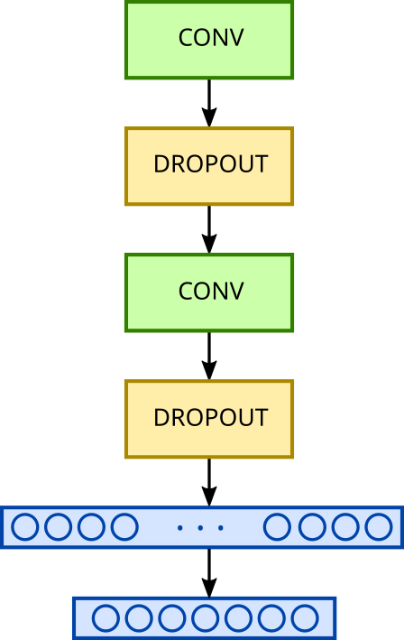
Basic convolution model
To train our network, we need to prepare the data so it can be fed into the network. We also need to divide the initial dataset into three sets: training, test, and validation.
## Learning part

### Generate data

encoded_list = []

for seq in df_human["sequence"]:
  encoded_list.append(cgr_encoding(seq, k =5))

X, y  = np.array(encoded_list), to_categorical(df_human["class"])

### Data spliting

X = X.reshape(4020, 32, 32, 1)

X_train, X_test, y_train, y_test = train_test_split(X, y, random_state = 42, stratify = y, shuffle = True, test_size = 0.2) # Split data into train and test with respect of class proportions

X_test, X_validation, y_test, y_validation = train_test_split(X_test, y_test, random_state = 42, stratify = y_test, shuffle = True, test_size = 0.5) # Split data into test and validation with respect of class proportions
Network parametrization
As mentioned previously, we’ll be using a small convolutional network. Unlike the network used last time, this one will be based on 2D convolutional blocks, though the operation is similar. For a quick refresher on convolution, you can check out this article: How Convolutional Neural Networks Work.
Our network will thus comprise two convolutional blocks (each consisting of a convolutional layer followed by a pooling layer, which is then followed by a dropout layer). These will be succeeded by a first dense layer that flattens the filters previously obtained by convolution, and then a dense layer with 7 neurons for classification.
Unlike last time, the classification layer will not use the sigmoid function for activation, but rather the softmax function to output a probability of belonging to a given class, rather than a “yes/no” type response.
Regarding optimization parameters, we’ll use an ADAM gradient descent (for adjusting network weights) with a learning rate of 0.001. The loss function will be “categorical cross entropy” to account for errors in a multi-class classification context.
The code required to build and train the network is as follows:
model = tf.keras.Sequential()

model.add(Conv2D(filters = 32, kernel_size = 3, activation = 'relu', padding = "valid", input_shape = (32, 32, 1), name = "Conv_1")) # Input shape : Batch_size, width, height, channels
model.add(Dropout(0.3, name = "Dropout_1"))
model.add(MaxPool2D(pool_size=4, strides=None, padding='valid', name = "MaxPool_1"))
model.add(Conv2D(filters = 64, kernel_size = 2, activation = 'relu', padding = "valid", name = "Conv_2")) # Input shape : Batch_size, width, height, channels
model.add(Dropout(0.3, name = "Dropout_2"))
model.add(tf.keras.layers.Flatten(name = "Flatten"))
model.add(tf.keras.layers.Dense(units = 7, activation = 'softmax', name = "Output"))

model.summary()
Model: "model"

┏━━━━━━━━━━━━━━━━━━━━━━━━━━━━━━━━━┳━━━━━━━━━━━━━━━━━━━━━━━━┳━━━━━━━━━━━━━━━┓
┃ Layer (type)                    ┃ Output Shape           ┃       Param # ┃
┡━━━━━━━━━━━━━━━━━━━━━━━━━━━━━━━━━╇━━━━━━━━━━━━━━━━━━━━━━━━╇━━━━━━━━━━━━━━━┩
│ Conv_1 (Conv2D)                 │ (None, 30, 30, 32)     │           320 │
├─────────────────────────────────┼────────────────────────┼───────────────┤
│ Dropout_1 (Dropout)             │ (None, 30, 30, 32)     │             0 │
├─────────────────────────────────┼────────────────────────┼───────────────┤
│ MaxPool_1 (MaxPooling2D)        │ (None, 7, 7, 32)       │             0 │
├─────────────────────────────────┼────────────────────────┼───────────────┤
│ Conv_2 (Conv2D)                 │ (None, 6, 6, 64)       │         8,256 │
├─────────────────────────────────┼────────────────────────┼───────────────┤
│ Dropout_2 (Dropout)             │ (None, 6, 6, 64)       │             0 │
├─────────────────────────────────┼────────────────────────┼───────────────┤
│ Flatten (Flatten)               │ (None, 2304)           │             0 │
├─────────────────────────────────┼────────────────────────┼───────────────┤
│ Output (Dense)                  │ (None, 7)              │        16,135 │
└─────────────────────────────────┴────────────────────────┴───────────────┘

 Total params: 24,711 (96.53 KB)

 Trainable params: 24,711 (96.53 KB)

 Non-trainable params: 0 (0.00 B)
# Compile model
model.compile(loss='categorical_crossentropy',
              optimizer=tf.keras.optimizers.Adam(learning_rate=0.001),
              metrics=['accuracy'])

# Define early stopping to avoid overfitting

early_stop = keras.callbacks.EarlyStopping(monitor = 'val_accuracy', min_delta = 0.0005, patience=8,
                                           restore_best_weights=True )

# Learning from data
history = model.fit(X_train, y_train, batch_size = 8, validation_data= (X_test, y_test),epochs=200)
First results
## Plot results

plt.figure(figsize = (10,4))
plt.subplot(121)
plt.plot(history.epoch, history.history["loss"], 'g', label='Training loss')
plt.plot(history.epoch, history.history["val_loss"], 'b', label='Validation loss')
plt.title('Training loss')
plt.xlabel('Epochs')
plt.ylabel('Loss')
plt.legend()

plt.subplot(122)
plt.plot(history.epoch, history.history["accuracy"], 'r', label='Training accuracy')
plt.plot(history.epoch, history.history["val_accuracy"], 'orange', label='Validation accuracy')
plt.title('Training accuracy')
plt.xlabel('Epochs')
plt.ylabel('Accuracy')
plt.legend()
plt.savefig(working_folder + "base_modelpng")
plt.show()

### Save model

working_folder = "/content/drive/MyDrive/Sequences/"
model.save(working_folder + 'base_modle.h5')

### Model evaluation

loss, acc = model.evaluate(X_validation, y_validation, verbose=2)
print("Basic model, accuracy : {:5.2f}%".format(100 * acc))
>>> Basic model, accuracy : 76.62%
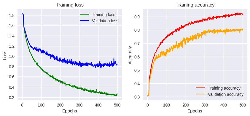
Base model training results
Our training is complete, what can we conclude?
The overall quality of the training is quite satisfactory. We’re reaching a plateau in accuracy, achieving 0.9 after 200 epochs (learning phases) during training. Validation accuracy is lower but acceptable. Our network seems to have learned quite well. Evaluating the model with the validation dataset gives us an overall performance of 76%, which is relatively good, but could we do better? Let’s see if transfer learning could help us.
Transfer Learning
Transfer learning involves using a previously acquired learning to address our current problem. However, we might be the first to pose this specific sequence classification question, especially considering our encoding based on chaos theory.
In practice, transfer learning is often implemented to address time and/or performance constraints. It involves reusing models similar to ours that have already been trained and deliver satisfactory results. You might ask how to find a model strictly identical to mine? Well, it’s not necessary for the model to be strictly identical. The input dimensions of the network simply need to be compatible with our data, or we can adapt our data to the pre-trained network.
This brings up the question of how the problem our network solves compares to the one the pre-trained network solves. To answer these questions, let’s dive directly into our example.
We’re going to use a convolutional network already trained on the MNIST dataset and adapt it to our needs. MNIST? You’ve probably come across it before; it’s that famous dataset containing images of handwritten digits, well-known in all deep learning tutorials. In principle, these images are of size 28x28x1. I’ve taken the liberty of adapting this network to accept our fractal representations of sequences, which have dimensions of 32x32x1. The network we’ll be using is an adaptation of the LeNet5 network proposed by Yann LeCun (more information available).
However, a major difference arises. The classification layer of this network has 10 neurons to account for an image of a digit belonging to a class between 0 and 9. Don’t panic, we’ll adapt this to our needs.
Let’s first train a fresh LeNet5 model on MNIST data with the 28x28x1 to 32x32x1 trick. We then plot the performances of the model and save it for later.
(x_train_lenet, y_train_lenet), (x_test_lenet, y_test_lenet) = mnist.load_data()

# Reshape data from (60_000, 28, 28) to (60_000, 32, 32) through zero-padding
x_train_lenet = np.pad(x_train_lenet, ((0,0),(2,2),(2,2)), 'constant')
x_test_lenet = np.pad(x_test_lenet, ((0,0),(2,2),(2,2)), 'constant')


# Peforming reshaping operation for model input
x_train_lenet = x_train_lenet.reshape(x_train_lenet.shape[0], 32, 32, 1)
x_test_lenet = x_test_lenet.reshape(x_test_lenet.shape[0], 32, 32, 1)

# Normalization to have images pixels in [0, 1]
x_train_lenet = x_train_lenet / 255
x_test_lenet = x_test_lenet / 255

# One Hot Encoding
y_train_lenet = keras.utils.to_categorical(y_train_lenet)
y_test_lenet = keras.utils.to_categorical(y_test_lenet)

# Building the Model Architecture
model_lenet = tf.keras.Sequential()


model_lenet.add(Conv2D(6, kernel_size=(5, 5), activation='relu', input_shape=(32, 32, 1)))

model_lenet.add(MaxPooling2D(pool_size=(2, 2)))

model_lenet.add(Conv2D(16, kernel_size=(5, 5), activation='relu'))

model_lenet.add(MaxPooling2D(pool_size=(2, 2)))

model_lenet.add(Flatten())
model_lenet.add(Dense(120, activation='relu'))

model_lenet.add(Dense(84, activation='relu'))

model_lenet.add(Dense(10, activation='softmax'))

model_lenet.summary()
As you can observe on the table below, all the parmeters of the model are trainable.
Model: "model_lenet"

┏━━━━━━━━━━━━━━━━━━━━━━━━━━━━━━━━━┳━━━━━━━━━━━━━━━━━━━━━━━━┳━━━━━━━━━━━━━━━┓
┃ Layer (type)                    ┃ Output Shape           ┃       Param # ┃
┡━━━━━━━━━━━━━━━━━━━━━━━━━━━━━━━━━╇━━━━━━━━━━━━━━━━━━━━━━━━╇━━━━━━━━━━━━━━━┩
│ conv2d_2 (Conv2D)               │ (None, 28, 28, 6)      │           156 │
├─────────────────────────────────┼────────────────────────┼───────────────┤
│ max_pooling2d_2 (MaxPooling2D)  │ (None, 14, 14, 6)      │             0 │
├─────────────────────────────────┼────────────────────────┼───────────────┤
│ conv2d_3 (Conv2D)               │ (None, 10, 10, 16)     │         2,416 │
├─────────────────────────────────┼────────────────────────┼───────────────┤
│ max_pooling2d_3 (MaxPooling2D)  │ (None, 5, 5, 16)       │             0 │
├─────────────────────────────────┼────────────────────────┼───────────────┤
│ flatten_1 (Flatten)             │ (None, 400)            │             0 │
├─────────────────────────────────┼────────────────────────┼───────────────┤
│ dense_3 (Dense)                 │ (None, 120)            │        48,120 │
├─────────────────────────────────┼────────────────────────┼───────────────┤
│ dense_4 (Dense)                 │ (None, 84)             │        10,164 │
├─────────────────────────────────┼────────────────────────┼───────────────┤
│ dense_5 (Dense)                 │ (None, 10)             │           850 │
└─────────────────────────────────┴────────────────────────┴───────────────┘

 Total params: 61,706 (241.04 KB)

 Trainable params: 61,706 (241.04 KB)

 Non-trainable params: 0 (0.00 B)
We want to keep all the layers of the network, and also benefit from the weights already pre-established by the previous training. However, the network isn’t ready for immediate use with our problem. We’ll need to “fine-tune” this model to leverage the descriptors (filters) established during training on the MNIST database, by only training (adjusting the weights of) a subset of our network’s layers. In our example, LeNet being a rather small model, we’ll keep the filters from all the layers except the first one. This means we’ll need to “freeze” the weights (coefficients of the convolutional filters) of the first layer and allow the network to adjust only the other layers’ weights.
Furthermore, we mentioned that LeNet5 allows for classification in a 10-class context. We’ll therefore remove the last layer of the network, whose role is to perform this classification, and replace it with a dense classification layer with 7 classes adapted to our problem, which will then be trained. We’ll keep the same optimization parameters as our first network: ADAM with a learning rate of 0.001, and a “categorical cross entropy” loss function.
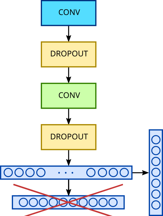
Scheme of LeNet5 fine-tuning process
The code required to perform these operations is as follows:
### Freeze bottom layers for transfer learning

# Freeze the first layers
for idx, layer in enumerate(lenet_model.layers):
  if idx <= 1 :
    layer.trainable = False

### Pop last dense layer and replace it for relevent goal

# Remove last layer
lenet_model.pop()

# Replace it with a more appropriate
lenet_model.add(tf.keras.layers.Dense(units = 7, activation = 'softmax', name = "Output"))

### Check modified model

lenet_model.summary()
Model: "lenet_model"

┏━━━━━━━━━━━━━━━━━━━━━━━━━━━━━━━━━┳━━━━━━━━━━━━━━━━━━━━━━━━┳━━━━━━━━━━━━━━━┓
┃ Layer (type)                    ┃ Output Shape           ┃       Param # ┃
┡━━━━━━━━━━━━━━━━━━━━━━━━━━━━━━━━━╇━━━━━━━━━━━━━━━━━━━━━━━━╇━━━━━━━━━━━━━━━┩
│ conv2d (Conv2D)                 │ (None, 28, 28, 6)      │           156 │
├─────────────────────────────────┼────────────────────────┼───────────────┤
│ max_pooling2d (MaxPooling2D)    │ (None, 14, 14, 6)      │             0 │
├─────────────────────────────────┼────────────────────────┼───────────────┤
│ conv2d_1 (Conv2D)               │ (None, 10, 10, 16)     │         2,416 │
├─────────────────────────────────┼────────────────────────┼───────────────┤
│ max_pooling2d_1 (MaxPooling2D)  │ (None, 5, 5, 16)       │             0 │
├─────────────────────────────────┼────────────────────────┼───────────────┤
│ flatten (Flatten)               │ (None, 400)            │             0 │
├─────────────────────────────────┼────────────────────────┼───────────────┤
│ dense (Dense)                   │ (None, 120)            │        48,120 │
├─────────────────────────────────┼────────────────────────┼───────────────┤
│ dense_1 (Dense)                 │ (None, 84)             │        10,164 │
├─────────────────────────────────┼────────────────────────┼───────────────┤
│ Output (Dense)                  │ (None, 7)              │           595 │
└─────────────────────────────────┴────────────────────────┴───────────────┘

 Total params: 61,453 (240.05 KB)

 Trainable params: 61,295 (239.43 KB)

 Non-trainable params: 156 (624.00 B)

 Optimizer params: 2 (12.00 B)
Now as you can see, only the 156 weights of the first layer are unfrozen and so, untrainable. The 61,295 other weights of the model are then retrained.
### Compile model and train

lenet_model.compile(loss='categorical_crossentropy',
              optimizer=tf.keras.optimizers.Adam(learning_rate=0.001),
              metrics=['accuracy'])

# Define early stopping to avoid overfitting
early_stop = keras.callbacks.EarlyStopping(monitor = 'val_accuracy', min_delta = 0.0005, patience=8,
                                           restore_best_weights=True )

history_lenet = lenet_model.fit(X_train, y_train, batch_size = 8, validation_data= (X_test, y_test),
                        epochs=200)

transfer_learning_directory = "/content/drive/MyDrive/Sequences/transfert_learning/"


lenet_model.save(transfer_learning_directory)
LeNet network analysis
Let’s look at our results:
"""# Plot final results"""

plt.figure(figsize = (14,4))
plt.subplot(121)
plt.plot(history.epoch, history.history["loss"], 'g', linestyle = 'dotted', label='Training - LeNet')
plt.plot(history_lenet.epoch, history_lenet.history["loss"], 'g', label='Training - LeNet')
plt.plot(history.epoch, history.history["val_loss"], 'b', label='Validation loss')
plt.plot(history_lenet.epoch, history_lenet.history["val_loss"], 'b' , linestyle = 'dotted', label='Validation  - LeNet')
plt.title('Training loss')
plt.xlabel('Epochs')
plt.ylabel('Loss')
plt.legend()

plt.subplot(122)
plt.plot(history.epoch, history.history["accuracy"], 'r', label='Training accuracy')
plt.plot(history_lenet.epoch, history_lenet.history["accuracy"], 'r',linestyle = 'dotted', label='Training - LeNet')

plt.plot(history.epoch, history.history["val_accuracy"], 'orange', label='Validation accuracy')
plt.plot(history_lenet.epoch, history_lenet.history["val_accuracy"], 'orange', linestyle = 'dotted', label='Validation - LeNet')

plt.title('Training accuracy')
plt.xlabel('Epochs')
plt.ylabel('Accuracy')
plt.legend()
plt.savefig(transfer_learning_directory + "dna_lenet_model.png")
plt.show()

"""### Evaluate model"""

loss, acc = lenet_model.evaluate(X_validation, y_validation, verbose=2)
print("DNA LeNet model, accuracy : {:5.2f}%".format(100 * acc))
>>> DNA LeNet model, accuracy : 70.15%
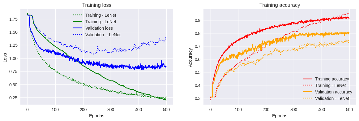
Results of LeNet5 fine-tuning
Here, we note two differences from the previous model. The first is that the accuracy at the end of our 500 epochs is slightly higher when using our DNA-LeNet. The validation accuracy is similar. However, the loss function value towards the end of training seems to behave erratically for this same network.
Furthermore, we observe a small plateau at the beginning of the training for both our models. However, the plateau in the case of our DNA-LeNet is shorter; the network starts learning more quickly but learns more slowly than our first network version.
Evaluating this new model with the validation dataset, we achieve an overall performance of 70.15%. It seems that changing models has barely helped us. Beyond the accuracy improvment, this was for illustrative and practical purpose.
Perhaps this is attributable to our classification layer struggling to deduce the correct class from all the features provided by the convolutional layers? Let’s see if we can classify our sequences differently than via this layer.
Coupling Deep Learning and Machine Learning
Unlike traditional machine learning, deep learning offers the advantage of partially freeing us from the need to extract features from our data. Indeed, in the context of a convolutional network, these features are learned. They are the convolutional filters whose coefficients are adjusted throughout the training.
Could we then keep only these features and provide them to a more conventional classification algorithm? That’s what we’re about to explore.
We’ll use SVM (Support Vector Machine). This is a binary classification algorithm whose general principle is quite simple. It involves placing our data in a high-dimensional vector space to establish the equation of a hyperplane, which will represent the boundary best separating the different classes associated with the various points in this space. In our case, this means separating the representations of different sequence classes by maximizing the margin between these representations.
Since it’s a separating hyperplane, we can only separate two classes at a time. Nevertheless, SVMs offer a strategy called “one vs one” that allows for building a multi-class classification system. Class separation will therefore occur pairwise in our space, aiming first to separate class 0 from class 1, then class 0 from class 2, then class 0 from class 3, and so on. We will then train as many binary classifiers as there are combinations of classes.
Once these classifiers are trained, the classification step will proceed as follows: A representation will be placed in the classification space. A class will be attributed according to each of the calculated hyperplanes. For a given representation, we will thus have a set of plausible classes. The predicted class will then be determined by majority vote. In other words, if class 0 is predicted 9 times, class 1 is predicted 3 times, and class 5 is predicted 5 times, then class 0 will be assigned to our representation.
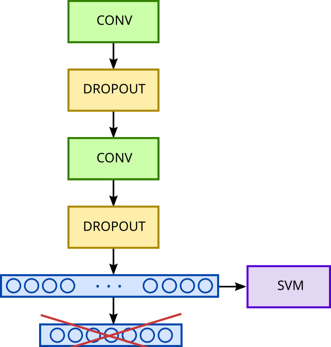
Coupling Between a CNN and an SVM
Enough theory, let’s get practical!
First, we need to transform our initial convolutional network into a feature extractor. To do this, we’ll remove the classification layer. The network’s output will then be the output of the “Flatten” layer, resulting in a 2304-dimensional vector per sequence.
## Change classification layer for SVM

### Adapt intial CNN for SVM classification

# Chop off head of CNN

svm_coupled_model = model
svm_coupled_model.pop()
svm_coupled_model.summary()
Model: "svm_coupled_model"

┏━━━━━━━━━━━━━━━━━━━━━━━━━━━━━━━━━┳━━━━━━━━━━━━━━━━━━━━━━━━┳━━━━━━━━━━━━━━━┓
┃ Layer (type)                    ┃ Output Shape           ┃       Param # ┃
┡━━━━━━━━━━━━━━━━━━━━━━━━━━━━━━━━━╇━━━━━━━━━━━━━━━━━━━━━━━━╇━━━━━━━━━━━━━━━┩
│ Conv_1 (Conv2D)                 │ (None, 30, 30, 32)     │           320 │
├─────────────────────────────────┼────────────────────────┼───────────────┤
│ Dropout_1 (Dropout)             │ (None, 30, 30, 32)     │             0 │
├─────────────────────────────────┼────────────────────────┼───────────────┤
│ MaxPool_1 (MaxPooling2D)        │ (None, 7, 7, 32)       │             0 │
├─────────────────────────────────┼────────────────────────┼───────────────┤
│ Conv_2 (Conv2D)                 │ (None, 6, 6, 64)       │         8,256 │
├─────────────────────────────────┼────────────────────────┼───────────────┤
│ Dropout_2 (Dropout)             │ (None, 6, 6, 64)       │             0 │
├─────────────────────────────────┼────────────────────────┼───────────────┤
│ Flatten (Flatten)               │ (None, 2304)           │             0 │
└─────────────────────────────────┴────────────────────────┴───────────────┘

 Total params: 58,000 (226.57 KB)

 Trainable params: 8,576 (33.50 KB)

 Non-trainable params: 0 (0.00 B)

 Optimizer params: 49,424 (193.07 KB)
The next step involves re-encoding the output data. We’ll feed all of our CGR (Chaos Game Representation) images into our network to obtain the corresponding vectors for the training, test, and validation sets:
### Prepare data for svm
# Go back on labels from one hot encoding
X_train_svm  = svm_coupled_model.predict(X_train)
y_train_svm = np.argmax(y_train, axis=1)

X_test_svm = svm_coupled_model.predict(X_test)
y_test_svm = np.argmax(y_test, axis=1)

X_validation_svm = svm_coupled_model.predict(X_validation)
y_validation_svm = np.argmax(y_validation, axis=1)

### Checking dimensions

print(f"Shape of x_train_svm : {X_train_svm.shape}")
print(f"Shape of y_train_svm : {y_train_svm.shape}")

print(f"Shape of x_test_svm : {X_test_svm.shape}")
print(f"Shape of y_test_svm : {y_test_svm.shape}")

print(f"Shape of x_validation_svm : {X_validation_svm.shape}")
print(f"Shape of y_validation_svm : {y_validation_svm.shape}")
>>> Shape of x_train_svm : (3216, 2304)
>>> Shape of y_train_svm : (3216,)
>>> Shape of x_test_svm : (402, 2304)
>>> Shape of y_test_svm : (402,)
>>> Shape of x_validation_svm : (402, 2304)
>>> Shape of y_validation_svm : (402,)
Finally, we’ll define our classifier, an SVM in “one vs one” mode, and train this model:
### Instanciate SVM classifier and train it

SVM_classifier = SVC(decision_function_shape = 'ovo', class_weight = "balanced", C = 125.0)
SVM_classifier.fit(X_train_svm, y_train_svm,)
Now that our model is trained using the features extracted by the modified initial convolutional network, let’s examine the results.
CNN - SVM coupling results analysis
### Evaluate classification

# Make predictions on test set

y_pred_svm = SVM_classifier.predict(X_test_svm)

accuracy = accuracy_score(y_test_svm, y_pred_svm)

## Confusion matrix

class_names = np.arange(7)

# Plot non-normalized confusion matrix
titles_options = [
    ("Confusion matrix, without normalization", None),
    ("Normalized confusion matrix", "true"),
]
for title, normalize in titles_options :
    disp = ConfusionMatrixDisplay.from_estimator(
        SVM_classifier,
        X_test_svm,
        y_test_svm,
        display_labels=class_names,
        cmap=plt.cm.Blues,
        normalize=normalize,
    )
    disp.ax_.set_title(title)
    plt.grid(False)

plt.grid(False)

plt.savefig(working_folder + "svm_confusion_matrix.png", bbox_inches='tight')
plt.show()

print(f"Acuracy using CNN coupled to SVM : {accuracy}")
>>> Acuracy using CNN coupled to SVM : 0.845771144278607
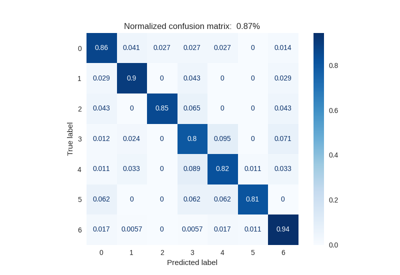
Confusion Matrix after CNN-SVM Coupled Prediction
As with any machine learning procedure, it was necessary to parameterize the model’s hyperparameters. Here, I only focused on the “C” coefficient, which is the margin coefficient for an SVM-type classifier.
The results here are very interesting. We obtain an accuracy of 84.6% compared to approximately 70-75% with our two previous approaches.
Observing the confusion matrix, we can see that classes 0, 1, and 6 are well separated from the others, while classes 2 and 3 seem more difficult to distinguish. Nevertheless, our classification system coupling CNN and SVM appears effective.
Conclusion
Throughout this tutorial, we’ve walked through the standard chain of a (mini) analysis based on machine learning.
The first step involved data import, an exploratory data analysis, and their encoding using chaos game theory. In a second step, we trained a small convolutional network with our sequences transformed into images.
In a third step, we attempted to improve the performance of this model by using another model of the same kind, trained on digit images, to address the concept of transfer learning.
It seems that the classification steps of these two previous networks struggled to fulfill their role. This might potentially be linked to the training, for which 200 epochs may not have been sufficient. Indeed, we can observe from the learning curves that the plateau isn’t fully reached.
Finally, in a last step, we sought to improve our classifier by using our initial convolutional network as a feature extractor and performing the classification with a Support Vector Machine, thus addressing the coupling of deep learning and machine learning.
All data, scripts, notebooks, and model saves are available in this git repository.
N.B.: If you reproduce this tutorial, your results may differ from those presented here due to the stochastic nature of the learning procedures and the initial dataset splitting.