Bioinformatics and AI: A First Step
Published:
The corresponding notebook about the following article can directly be launched through google collab ![]()

DNA matrix genetics | TheDigitalArtist
Artificial Intelligence, Machine Learning, Deep Learning: What About the Data Scientist?
Artificial Intelligence (AI), Machine Learning, Deep Learning – these terms feel both foreign and familiar at the same time… How do you find your way through this jungle of technical terms?
Let’s start by defining what AI is. A basis for science fiction for some, a source of concern for others, we’ll approach AI from a technical perspective. Inspired by biology and cognitive sciences, and built on mathematical foundations, artificial intelligence is defined as a set of algorithms designed to replicate decisions made by a human being to accomplish a specific task.
“Human” implies perceptual learning, memory organization, and critical reasoning. Indeed, any AI algorithm will require human knowledge, both in the preparation and labeling of data, and in its interpretation. —
AI, but for what purpose?
The tasks that AI can accomplish are as varied as the definition of AI itself, and as diverse as the number of approaches to solve a given problem. The most commonly solved tasks using artificial intelligence include: classification (binary, multi-class), regression, image segmentation (automated identification of different image components), data denoising, object detection, natural language processing, etc. (this list is not exhaustive). For more general information on deep learning and its applications, click here.
Now, let’s roll up our sleeves and tackle our first AI project.
Defining the Problem
For this introduction, we’ll address a relatively simple problem using simple data. Today, we’re focusing on the classification of DNA sequences to determine whether these sequences are promoters or not (binary classification). The idea is to feed a nucleotide sequence into our network and get a 0 or 1 output, representing non-promoter and promoter characteristics of our sequence respectively (0: the sequence is not a promoter, 1: it is). The data will be divided into two files: one containing promoter sequences, the other containing non-promoter sequences. Data available here, the code notebook is available there.
Data Preparation
For this project, though not overly complex, we’ll use Google Colab to easily access data and benefit from sufficient resources. Of course, you can reproduce this process locally, and perhaps even with better performance.
Let’s start by “mounting” our Drive so we can access the data, define the necessary paths, and import the required libraries.
from google.colab import drive
import numpy as np
import pandas as pd
import matplotlib.pyplot as plt
import  tensorflow as tf
import keras
from keras.layers import Dense, Dropout, Flatten, Conv1D, MaxPooling1D
from keras import regularizers
from keras.callbacks import EarlyStopping, ModelCheckpoint
from keras.wrappers.scikit_learn import KerasClassifier
from sklearn.model_selection import train_test_split

# mount google drive
drive.mount('/content/drive')

# Paths definitions
work_folder = "/content/drive/MyDrive/Promoters_classification/"
non_promoters_set = work_folder + "NonPromoterSequence.txt"
promoter_set = work_folder + "PromoterSequence.txt"
The data isn’t in a “standard” format for common libraries, so we’ll need to format it correctly. Note that this is FASTA-type data, meaning the separator will be a chevron >. You can find an article from bioinfo-fr about the FASTA format here.
We want to transform this into a two-column table: sequence and label. Additionally, our data is currently in two separate files that we’ll need to combine. Let’s get that done.
# Load, sanitize and label non promoter sequences
df_non_promoters = pd.read_csv(non_promoters_set, sep = '>', )
df_non_promoters.dropna(subset=['Unnamed : 0'], how='all', inplace=True)
df_non_promoters.reset_index(inplace = True)
df_non_promoters.drop(['EP 1 (+) mt:CoI_1 ; range -400 to -100.', 'index'], axis = 1, inplace=True) #data cleaning after error found
df_non_promoters.rename(columns={'Unnamed : 0': "sequence"}, inplace = True)
df_non_promoters['label'] = 0
# Load, sanitize and label non promoter sequences
df_promoters = pd.read_csv(promoter_set, sep = '>', )
df_promoters.dropna(subset=['Unnamed : 0'], how='all', inplace=True)
df_promoters.reset_index(inplace = True)
df_promoters.drop(['EP 1 (+) mt:CoI_1 ; range -100 to 200.', 'index'], axis = 1, inplace=True) #data cleaning after error found
df_promoters.rename(columns={'Unnamed : 0': "sequence"}, inplace = True)
df_promoters['label'] = 1
# Concatenate the two frames
df = pd.concat([df_non_promoters, df_promoters], axis = 0 )
print(f"Shape of the full dataset : {df.shape}")

>>> Shape of the full dataset : (22600, 2)
>>>                                             sequence  label
>>> 0  TAATTACATTATTTTTTTATTTACGAATTTGTTATTCCGCTTTTAT...      0
>>> 1  ATTTTTACAAGAACAAGACATTTAACTTTAACTTTATCTTTAGCTT...      0
>>> 2  AGAGATAGGTGGGTCTGTAACACTCGAATCAAAAACAATATTAAGA...      0
>>> 3  TATGTATATAGAGATAGGCGTTGCCAATAACTTTTGCGTTTTTTGC...      0
>>> 4  AGAAATAATAGCTAGAGCAAAAAACAGCTTAGAACGGCTGATGCTC...      0
We now have a two-column table containing 22,600 sequences and their corresponding labels. Like any good data analysis, it’s essential to clean this data. In our case, this means removing sequences that contain nucleotides marked as “N.”
nb_sequences_to_drop = 0
rows_indexes_to_drop = list()
for idx, seq in enumerate(df['sequence']):
    if 'N' in seq :
      nb_sequences_to_drop +=1
      # display(df.loc[df['sequence'] == seq])
      rows_indexes_to_drop.append(idx)
print(f"Number of sequence to be dropped : {nb_sequences_to_drop}")
print(f"Rows to be dropped : {rows_indexes_to_drop}")
print(f"Shape of the data before dropping sequences containing Ns : {df.shape}")
df.drop(rows_indexes_to_drop, inplace = True)
print(f"Shape of the data after dropping sequences containing Ns : {df.shape}")

>>> Number of sequences to be dropped : 1
>>> Rows to be dropped : [1822]
>>> Shape of the data before dropping sequences containing Ns : (22600, 2)
>>> Shape of the data after dropping sequences containing Ns : (22598, 2)
We’re going to build a convolutional network based on textual data. Since this type of network can’t directly process text data, we’ll need to change its representation. A classic way to do this is by using a “one-hot encoding” strategy.
DNA sequences encoding
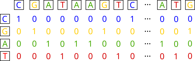
The idea is to characterize (for our problem) each base in the sequence using a quadruplet of values that are either 0 or 1, with only one value being 1. Thus, the four bases are encoded as: A: {1, 0, 0, 0}, T: {0, 1, 0, 0}, C: {0, 0, 1, 0}, and G: {0, 0, 0, 1}.
In our case, since our sequences are 301 nucleotides long, this transformation will result in a matrix of size 4 x 301 for a single sequence. At the dataset level, the dimensions will be 22598 x 301 x 4. Let’s perform our encoding.
sequence = list(df.loc[:, 'sequence'])
encoded_list = []
def encode_seq(s):
    Encode = {'A':[1,0,0,0],'T':[0,1,0,0],'C':[0,0,1,0],'G':[0,0,0,1]}
    return [Encode[x] for x in s]
for i in sequence :
    x = encode_seq(i)
    encoded_list.append(x)
X = np.array(encoded_list)
print(f" Shape of one-hot encoded sequences : {X.shape}")

>>> Shape of one-hot encoded sequences : (22598, 301, 4)
Our data is now almost ready. The next step is to separate the transformed sequences from their labels.
Preparing Training, Test, and Validation Datasets
Now, it’s necessary to split our data into three subsets: training, testing, and validation. The training data will allow the network to adjust its weights based on the error between its prediction (promoter or non-promoter sequence type) and the actual label. The test data will be used to evaluate the performance of the training, and finally, the validation data will give us the model’s performance once it’s trained.
All three datasets must be independent of each other to ensure we don’t encounter a sequence example already seen during training. It’s also necessary to ensure (if possible) that each set has equal proportions of the different classes. Let’s prepare our datasets.
# Reshape data to allow network processing
X = X.reshape(X.shape[0],301, 4, 1) # Tensor containing one-hot encoded sequences wich are promotors or not
y = df['label'] # Tensor containing labels for each sequence (0 : sequence is nt a promotor, 1 : sequence is a promotor)
print(y.value_counts())
print(f"Shape of tensor containing sequences one-hot encoded {X.shape}n")
print(f"Shape of tensor containing labels relatives to the sequences : {y.shape}")

>>> 0    11299
>>> 1    11299
>>> Name : label, dtype : int64
>>> Shape of tensor containing sequences one-hot encoded (22598, 301, 4, 1)
>>> Shape of tensor containing labels relatives to the sequences : (22598,)
We need to ensure that we have the same number of sequences as labels. Since that’s the case, let’s proceed with stratified division of our data.
Model Construction
To answer our question, we’re going to build a shallow convolutional neural network, with an output layer having only a single neuron. If this neuron is activated, it indicates that the sequence is a promoter type. To learn more about convolutional networks, I recommend this video.
Is Learning an Optimization Problem?
Learning problems, whether deep or machine learning, can be defined as optimization problems. This involves constructing a system or model that is initially “naive,” which we then train. In our case, the goal is to make our model increasingly effective by training it to correctly classify promoter sequences from non-promoter sequences. To do this, we’ll repeatedly ask the network to classify a set of examples in batches and evaluate an error. This error will then be used to adjust the coefficients of the convolution kernels until an optimum is reached.
This optimum corresponds to the global minimum of the cost function (or Loss), which evaluates the amount of error made by the model in its classification tasks. We’ll then adjust these weights based on the intensity of this error: the higher the error, the more the coefficients will be modified; conversely, the smaller the error, the less the coefficients will be modified. This error is evaluated by calculating the gradient of the error function, or more formally, the partial derivative at each neuron in the network with respect to the neuron. This same error is weighted by the learning rate, which scales the strength of the weight modification. Thus, the lower the learning rate, the slower the training, but the more likely it is to converge towards a global optimum.
How to Define the Quantity of Error
The quantity of error is evaluated by the cost function (or Loss). This function reflects the number of incorrectly predicted classes when evaluating a set of training sequences. Depending on the problems to be solved, cost functions differ, particularly based on the number of possible classes and any existing relationships between these classes.
The quantity of error is evaluated with each prediction of sequence batches. The partial derivative of this error function will then be calculated with respect to each of the network’s parameters, in order to adjust them in the “opposite” direction of this derivative. Thus, when the quantity of errors stabilizes or reaches very low values, the adjustment of parameters is minimal, and learning could conclude.
In the examples below, the cost function used will be the “Binary Cross-Entropy,” which accounts for classification error in a two-class optimization problem.
You Said Convolution?
Convolution is a mathematical operation on matrices. It involves “matching” a matrix representing the data with a matrix called a “convolution kernel” (or filter). The resulting matrix is the matrix product between the data matrix and the kernel (to which a matrix containing the bias weights of each neuron is sometimes added).
DNA sequences encoding
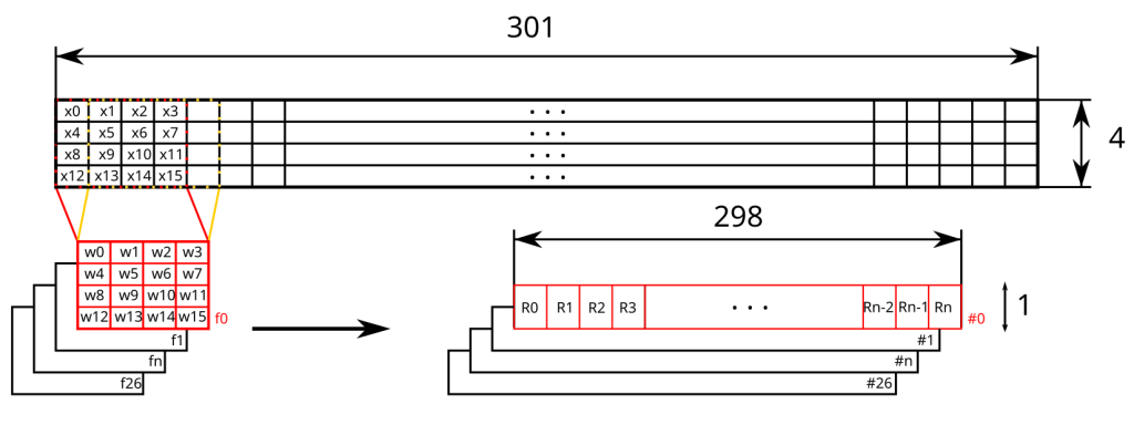
Based on the first convolution operation in the previous illustration, we would have:
\[R_{0} = \sum_{i = 0}^{15}w_ix_i\]This convolution operation is performed multiple times by sliding the kernel (in red) along the encoded sequence of dimension 301x4. Here, we’ll use “valid” padding, which only allows convolution when the kernel completely “covers” the sequence. This means the number of convolutions, and consequently the size of the output representation, will be limited to 298. Thus, filter f0 will slide with a stride of 1 across the sequence, resulting in 298 positions, leading to as many convolution operations. Ultimately, for this filter, the output dimension will be 298x1.
We then repeat the same operation for the 26 other filters, from f1 to f26. The output of this convolution layer will therefore be a representation with dimensions of 298x1x27.
This convolution result will then undergo an activation operation, which involves finding the image of each element of the resulting matrix (from the convolution) using the activation function (here, ReLU for “Rectified Linear Unit”). This operation aims to highlight the most relevant values/elements of the new representation after convolution, which will then be passed to the next layers of the network.
Pool!
Convolutional layers are followed by pooling layers. These layers aim to subsample the results of the convolutional layers to retain only the pertinent information from this representation, and also to reduce the size of the initial sequence’s representation as it passes through the network.
There are several methods for subsampling convolution results. The general idea is to select a single value from a more or less large set of contiguous values in the post-convolution representation. First, we need to define the size of this search window. In the example below, this size will be 3. Then, we choose the function or method to extract a single value from this window.
This choice could be the average of the window values, the median, the minimum, or in our case, the maximum.
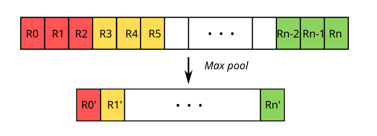
Illustration of max pooling
Thus, in our case, we’ll extract values of interest within a window sliding along the convolution result vector, with a window size of 3. We’ll use the max function, meaning we’ll only retain the maximum value for a window of 3 contiguous values before repeating the operation for the next three. More formally:
\[R'_0 = max(R_{0}, R_{1}, ..., R_{n})\]Thus, after subsampling with a window of size 3, the dimensions of our 27 post-convolution representations will be divided by 3.
The Concept of Receptive Fields
As we mentioned in the introduction, neural networks are inspired by biology. As we know, in the nervous system, neurons are connected in a cascade. Some neurons receive pre-processed information via the axons of their predecessors at the soma. Therefore, for a given neuron, the received signal compiles information transmitted by its predecessors, who themselves may have received condensed information from the perceptual system.
A parallel can be drawn with convolutional networks. The first convolutional block (convolution layer + activation + pooling) “sees” the entire input sequence. However, as we’ve just seen, the output of this first block is smaller in dimension than the input sequence, and it no longer carries biological meaning as such. The information transmitted is a condensed version of the initial sequence.
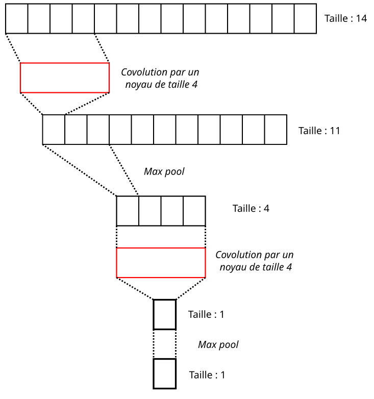
Illustration of receptor field
If we look at the example above, the sequence is of size 14. Performing a convolution with a kernel of size 4 results in an output representation of size 11. Then, we apply subsampling with a window of size 3, yielding an output representation of size 4 from the first convolutional block. In the next convolutional block, convolving this representation with a kernel of size 4 leads to a new representation of size 1, which after pooling with a window of size 3 also gives an output representation of size 1.
The reasoning remains the same as layers succeed each other: the representations decrease in size, and neurons further down a layer “see” an increasingly broader view of the input data. It’s worth noting that once their values are adjusted at the end of training, the convolution kernels can then extract key features from the input sequence crucial for determining the network’s output class. Furthermore, the deeper the layers are in the network, the more complex the extracted features will be.
First Attempt
In this initial experiment, we’ll use stochastic gradient descent, which is a basic optimizer.
Python

model = tf.keras.Sequential()
model.add(tf.keras.layers.Conv1D(filters = 27, kernel_size = 4, activation = 'relu', padding = "valid", input_shape = (X_train.shape[1], X_train.shape[2])))
model.add(tf.keras.layers.MaxPool1D(pool_size=3, strides=None, padding='valid'))
model.add(tf.keras.layers.Conv1D(filters = 14, kernel_size = 4, activation = 'relu'))
model.add(tf.keras.layers.MaxPool1D(pool_size= 2, strides = None, padding = 'valid'))
model.add(tf.keras.layers.Conv1D(filters = 7, kernel_size = 4, activation = 'relu'))
model.add(tf.keras.layers.MaxPool1D(pool_size= 2, strides = None, padding = 'valid'))
model.add(tf.keras.layers.Flatten())
model.add(tf.keras.layers.Dense(units = 1, activation = 'sigmoid'))
model.summary()
model.compile(loss='binary_crossentropy',
              optimizer='sgd',
              metrics=['accuracy'])
# We define an early stop for training in case of no significant improvement after several phases to avoid overfitting
early_stop = keras.callbacks.EarlyStopping(monitor = 'val_accuracy', min_delta = 0.0005, patience=8,
                                           restore_best_weights=True )

# We define a monitoring for the model's performance and launch the training
history = model.fit(X_train, y_train, batch_size = 128, validation_data=(X_test, y_test),
                        epochs=115)
# We plot the training results
plt.figure(figsize = (10,4))
plt.subplot(121)
plt.plot(history.epoch, history.history["loss"], 'g', label='Training loss')
plt.plot(history.epoch, history.history["val_loss"], 'b', label='Validation loss')
plt.title('Training loss')
plt.xlabel('Epochs')
plt.ylabel('Loss')
plt.legend()
plt.subplot(122)
plt.plot(history.epoch, history.history["accuracy"], 'r', label='Training accuracy')
plt.plot(history.epoch, history.history["val_accuracy"], 'orange', label='Validation accuracy')
plt.title('Training accuracy')
plt.xlabel('Epochs')
plt.ylabel('Accuracy')
plt.legend()
plt.savefig(work_folder + "base_model_deep_no_dropout_sgd.png")
plt.show()
We can observe several things from our learning curves. First, whether in training or validation, neither the loss nor the performance reaches a plateau. It seems that despite 150 training passes (epochs), the optimum hasn’t been reached.
NB: A pass (or epoch) corresponds to one training session of the model. At the end of the first epoch, all training examples have been seen once; at the end of epoch ‘n’, all these same examples have been seen ‘n’ times by the network.
Furthermore, we can observe that the validation performance, which is on examples not seen during training, is worse.
Our model therefore seems under-trained on one hand, and shows difficulty generalizing.
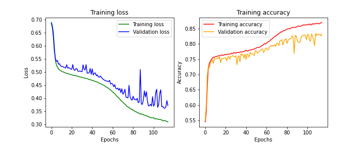
Results obtained with SGD optimizer
# Model final evaluation
loss, acc = model.evaluate(X_validation, y_validation, verbose=2)
print("Untrained model, accuracy : {:5.2f}%".format(100 * acc))

>>> 71/71 - 0s - loss : 0.3394 - accuracy : 0.8575 - 404ms/epoch - 6ms/step
>>> Untrained model, accuracy : 85.75%)
While the results aren’t perfect, the model achieves 85.75% accuracy, which is already quite good. Let’s see how we can improve our model’s performance using a different optimizer.
ADAM Optimizer
Let’s switch the SGD optimizer for an ADAM optimizer. This optimizer is based on the principles of SGD but utilizes the first and second-order moments of the error function’s gradient. This allows the optimizer to have a “memory” of previous training, and thus of the strength of prior modifications to the convolution kernel coefficients.
Furthermore, this type of optimizer incorporates an adaptive learning rate, which will allow for significant modifications to the convolution kernel coefficients at the beginning of training, and less forceful adjustments as the training phases progress.
Thus, our model will learn by taking into account more than just the immediate previous training step, and it will refine its learning more precisely over time.
model_adam = tf.keras.Sequential()
model_adam.add(tf.keras.layers.Conv1D(filters = 27, kernel_size = 4, activation = 'relu', padding = "valid", input_shape = (X_train.shape[1], X_train.shape[2])))
model_adam.add(tf.keras.layers.MaxPool1D(pool_size=3, strides=None, padding='valid'))
model_adam.add(tf.keras.layers.Conv1D(filters = 14, kernel_size = 4, activation = 'relu'))
model_adam.add(tf.keras.layers.MaxPool1D(pool_size= 2, strides = None, padding = 'valid'))
model_adam.add(tf.keras.layers.Conv1D(filters = 7, kernel_size = 4, activation = 'relu'))
model_adam.add(tf.keras.layers.MaxPool1D(pool_size= 2, strides = None, padding = 'valid'))
model_adam.add(tf.keras.layers.Flatten())
model_adam.add(tf.keras.layers.Dense(units = 1, activation = 'sigmoid'))
model_adam.summary()
model_adam.compile(loss='binary_crossentropy',
              optimizer='adam',
              metrics=['accuracy'])
early_stop = keras.callbacks.EarlyStopping(monitor = 'val_accuracy', min_delta = 0.0005, patience=8,
                                           restore_best_weights=True )


history_adam = model_adam.fit(X_train, y_train, batch_size = 128, validation_data=(X_test, y_test),
                        epochs=115)
plt.figure(figsize = (10,4))
plt.subplot(121)
plt.plot(history_adam.epoch, history_adam.history["loss"], 'g', label='Training loss')
plt.plot(history_adam.epoch, history_adam.history["val_loss"], 'b', label='Validation loss')
plt.title('Training loss')
plt.xlabel('Epochs')
plt.ylabel('Loss')
plt.legend()
plt.subplot(122)
plt.plot(history_adam.epoch, history_adam.history["accuracy"], 'r', label='Training accuracy')
plt.plot(history_adam.epoch, history_adam.history["val_accuracy"], 'orange', label='Validation accuracy')
plt.title('Training accuracy')
plt.xlabel('Epochs')
plt.ylabel('Accuracy')
plt.legend()
plt.savefig(work_folder + "base_model_deep_no_dropout_adam.png")
plt.show()
The ADAM optimizer is known for converging more quickly (reaching the global minimum of the cost function), but on the other hand, it can struggle to generalize.
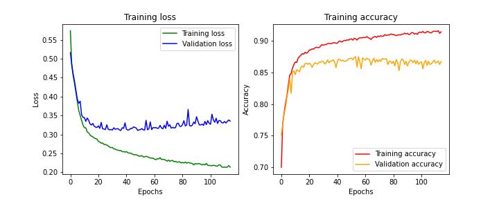
Results obtained with ADAM optimizer
# Final evaluation
loss, acc = model_adam.evaluate(X_validation, y_validation, verbose=2)
print("Untrained model, accuracy : {:5.2f}%".format(100 * acc))

>>> 71/71 - 0s - loss : 0.3810 - accuracy : 0.8509 - 496ms/epoch - 7ms/step
Untrained model, accuracy : 85.09%
We can observe that the model’s performance hovers around 85% accuracy. Nevertheless, both the loss and accuracy curves seem to have plateaued, indicating that the training appears to have run its course. However, we note that the validation loss is higher (and respectively, validation accuracy is lower) than during training. Once again, the model generalizes less effectively on unseen examples. Furthermore, we observe an increase in validation loss beyond the 60th epoch. This is a clear sign of overfitting, where the model learns too well on its training data, causing performance to drop when new examples are presented.
Let’s now explore how to remedy this overfitting issue.
model_adam_dropout = tf.keras.Sequential()
model_adam_dropout.add(tf.keras.layers.Conv1D(filters = 27, kernel_size = 4, activation = 'relu', padding = "valid", input_shape = (X_train.shape[1], X_train.shape[2])))
model_adam_dropout.add(tf.keras.layers.MaxPool1D(pool_size=3, strides=None, padding='valid'))
model_adam_dropout.add(tf.keras.layers.Dropout(0.2)) # Add a Dropout layer
model_adam_dropout.add(tf.keras.layers.Conv1D(filters = 14, kernel_size = 4, activation = 'relu'))
model_adam_dropout.add(tf.keras.layers.MaxPool1D(pool_size= 2, strides = None, padding = 'valid'))
model_adam_dropout.add(tf.keras.layers.Dropout(0.2)) # Add a Dropout layer
model_adam_dropout.add(tf.keras.layers.Conv1D(filters = 7, kernel_size = 4, activation = 'relu'))
model_adam_dropout.add(tf.keras.layers.MaxPool1D(pool_size= 2, strides = None, padding = 'valid'))
model_adam_dropout.add(tf.keras.layers.Dropout(0.2)) # Add a Dropout layer
model_adam_dropout.add(tf.keras.layers.Flatten())
model_adam_dropout.add(tf.keras.layers.Dense(units = 1, activation = 'sigmoid'))
model_adam_dropout.summary()
model_adam_dropout.compile(loss='binary_crossentropy',
              optimizer='adam',
              metrics=['accuracy'])
# We define an early stop for training in case of no significant improvement after several phases to avoid overfitting
early_stop = keras.callbacks.EarlyStopping(monitor = 'val_accuracy', min_delta = 0.0005, patience=8,
                                           restore_best_weights=True )
It’s important to note that when the model is trained and making predictions, all neurons are connected. Dropout only applies during the learning process.
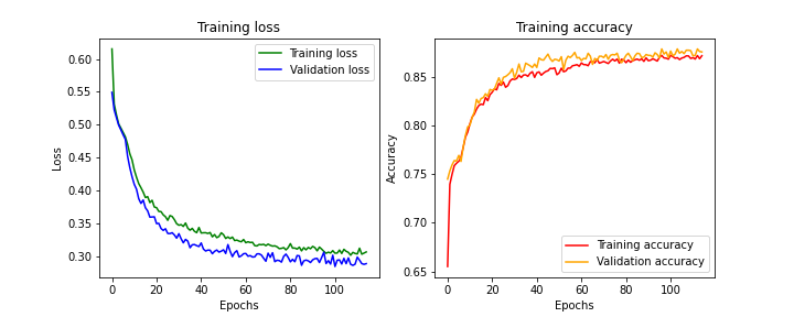
Effects of the droput on learning process
# Model final evaluation

loss, acc = model_adam_dropout.evaluate(X_validation, y_validation, verbose=2)
print("Untrained model, accuracy : {:5.2f}%".format(100 * acc))

>>> 71/71 - 0s - loss : 0.2720 - accuracy : 0.8819 - 365ms/epoch - 5ms/step
Untrained model, accuracy : 88.19%
We observe, as in the previous example, that both the loss and accuracy curves reach a plateau for both training and validation.
Furthermore, we no longer see a significant divergence between training and validation (in terms of both loss and accuracy) throughout the training process. This suggests that we’ve successfully trained the model without causing overfitting.
It’s worth noting that the final accuracy value is lower with the use of dropout (around 85%) than in the previous experiment (around 90%). However, when evaluating the model, performance actually increased from 85% for the previous model to 88% for this model.
Attempts to make models more generalizable sometimes come with a loss in performance. However, here we seem to have established a model with respectable performance.
Conclusion
This concludes a first experiment in applying deep learning to bioinformatics problems. We built a model capable of classifying 301-nucleotide sequences as either promoter or non-promoter.
We’ve seen that numerous hyperparameters come into play during model construction and training to make it more robust to new examples and to train it within reasonable timeframes.
It’s important to keep in mind that this network architecture isn’t the only one that can solve this problem, nor is it necessarily the best. Many possibilities exist to refine this model, both in terms of parameterization and architecture.
The complete code is available on this repo: https://github.com/bioinfo-fr/data_ia/blob/main/DNA_CNN_promoters.ipynb
To Go Further with Convolutional Networks
Here are some resources on CNNs: https://towardsdatascience.com/a-comprehensive-guide-to-convolutional-neural-networks-the-eli5-way-3bd2b1164a53